Next-Concept Modeling: a model that doesn't write word by word

A language model writing a 1,000-token answer runs itself 1,000 times, once per token, and no run can start until the previous one has finished. That’s how nearly every chatbot works today, and it’s why long answers and long reasoning chains take time.

A new paper from Stanford, Next-Concept Modeling: Fast, Parallel Coarse-to-Fine Text Generation (opens in a new tab), tries a different order. Its model, NCM, sketches the whole answer first and then adds detail in a few layers, filling in every position of a layer at once. For a 1,024-token passage, that’s 32 passes instead of 1,024. In the researchers’ tests it ran 10 to 31 times faster than diffusion language models, which also write in parallel, and it solved 86 percent of hard Sudoku puzzles. A left-to-right model trained for the same test solved about 1 percent.

9:54Prefer watching a video instead?Watch "NCM Explained: How AI Generates Text Beyond Word by Word" on YouTube. (opens in a new tab)

Three ways to write a sentence

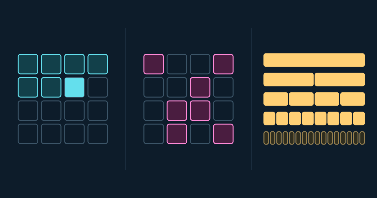
There are three orders worth comparing. A regular LLM is like laying bricks: left to right, one at a time. A diffusion model is more like a crossword: it fills in blanks across the whole text, a few per pass, over many passes. NCM is more like an architect: first a rough outline of the whole building, then the rooms, then the furniture, everywhere at once.

The figure below runs all three on the same sentence, one pass per tick. Watch the pass counters more than the words.

Why a language model can’t skip ahead

A regular LLM first splits your text into tokens and turns each one into a vector, a list of numbers. The vectors flow through dozens of layers, and in each layer every token looks back at the tokens before it. Your prompt goes through all at once, in parallel. Writing the answer is different. At the end of each run, the model scores every possible next token, picks one, appends it, and runs again for the token after that.

Each of those runs reads the model’s weights from GPU memory, and that’s the slow part. An H100 GPU has 80 GB of memory but only about 50 MB of fast on-chip storage, so the weights stream in layer by layer for every new token. Each weight then takes part in roughly one calculation before it makes room for the next layer. Performance studies (opens in a new tab) of this kind of decoding find the same thing: the math is quick, and moving the weights is what takes the time. Real serving systems batch many users together and cache earlier work, so this is a simplified picture, but the basic limit holds for each individual answer: one token per run.

How diffusion fills in the blanks

Diffusion took a different route. Image generators start from static and remove a little noise per step until a picture appears. Words can’t be made “a little noisy” in the same simple way, so a popular text version, masked diffusion (opens in a new tab), hides words behind a mask instead.

During training, the model sees real sentences with some of their words hidden, sometimes a few and sometimes almost all, and learns to fill them in using the words on both sides. When it writes, it starts with every word hidden. Each step guesses every hidden word at once, keeps the guesses it’s most sure about (opens in a new tab), and hides the rest again for the next step.

The weakness is that words guessed in the same step can’t see each other. Fill in too many at once and they clash, giving repeats like “the the the.” So diffusion models take many small steps. The baselines in the NCM paper used 128 steps, and up to 1,024 on longer passages.

NCM keeps the “all at once” part of diffusion. What it changes is what gets filled in first.

What NCM writes: codes in layers

NCM doesn’t predict words directly. It predicts codes, numbers that point to entries in a learned codebook. In most of the paper’s settings, each layer has its own codebook of 4,096 entries.

The codes come in layers. The top layer has only a few codes and carries the rough idea; the paper defines “concept” as the information in these coarse layers. Each layer below has more codes and adds more detail, until the last layer has one code per token. Depending on the task, the paper’s models use between 8 and 32 layers. A small decoder turns the final layers back into words.

Training: a tokenizer, then a generator

NCM is trained in two stages, both before it’s ever used.

The first stage trains what the paper calls a multiscale tokenizer. It isn’t the usual tokenizer that splits text into words; it works on those tokens and turns a passage into layers of codes. Every token becomes a vector, the passage is squeezed into a few vectors, and each is swapped for its closest codebook entry. That’s the top layer. The tokenizer then looks at what that sketch got wrong and encodes the difference with more codes, layer after layer. The codebook is learned at the same time: entries start out random, and each one is nudged toward the vectors that picked it until the entries settle into useful patterns. During training, the finer layers are sometimes dropped, which forces the top layers to carry the big picture on their own.

The result is close to lossless. Decoding all the layers rebuilds 99.99 percent of tokens on web text and 98.79 percent on the translation task.

Then the tokenizer is frozen, and the second stage trains the generator, a transformer that learns to predict each layer of codes from the layers above it. The authors list the separate stages as a limitation: training both parts together might work better.

Writing an answer, one layer at a time

A prompt is handled differently from the answer. It’s split into tokens the usual way and embedded with the frozen tokenizer, and the generator reads it as context; the prompt itself is never turned into layers. The answer starts empty.

In the first pass, the generator predicts every code in the top layer at once. Those codes are looked up in the codebook, and that sketch is the input for the next pass, which predicts the whole next layer. After the last layer, the decoder turns the codes into text.

The paper shows this on a German-to-English translation. After the first layer, the output is a mess of repeats, the same clash diffusion runs into, but the shape of the sentence is already there. “Medium-sized enterprises” appears by layer 4. By layer 8 it’s nearly right, and layer 11 is clean. The full trajectory also shows that quality doesn’t rise at every step: layer 9 scores lower than layer 8 before the final layers recover.

That’s the reason for the name. A regular model predicts the next token. NCM predicts the next layer of the concept, each one more detailed.

The number of passes depends on the number of layers, not the number of words. In the researchers’ code (opens in a new tab), the web-text model’s 32 layers grow as squares: 1 code, then 4, then 9, and so on up to 1,024. That’s 32 passes for a 1,024-token passage.

What the speedups measure

The speed results are the researchers’ own lab tests. They timed the generation of 1,024 passages, 16 at a time, on a single NVIDIA H100, against the strongest diffusion model for each task:

• News summarization (XSum): 31 times faster than AURORA-LM at matching quality, with 16 times fewer passes.
• Language modeling (LM1B): 21 times faster than DUO, with 11 times fewer passes and slightly better scores.
• Open-ended web text (OpenWebText): about 10 times faster, with competitive quality.

On the first two tasks, the speedup is bigger than the cut in passes, because each NCM pass costs less on average.

The researchers also spent the saved time on extra attempts. Generating several summaries and picking the best one gave about 7 percent higher scores than the strongest summarization baseline, in the same amount of time.

Training was cheaper too. On LM1B, NCM’s tokenizer and generator together processed 13.4 billion tokens, against 66 billion for the diffusion baselines, about 4.9 times fewer.

These speedups are all against diffusion models, not against regular left-to-right LLMs.

Where the speed comes from

A regular LLM reads all the weights for every token, and each read feeds only a little math, so it’s memory-heavy. Diffusion flips that: each step reads the weights once but works on the whole text, so it’s compute-heavy, and it repeats that for 128 steps or more.

NCM is compute-heavy too, since each pass works on a whole layer at once. But the top layers are small, so the first passes are cheap, and there are only a few dozen passes in total. Fewer reads of the weights, and less wasted math. Try changing the answer length and step counts below.

There’s an open question here. When a server handles many users at once, batching keeps a regular LLM’s cores busy too, because each weight it reads serves many answers. NCM’s advantage could shrink on busy servers. The paper timed only one batch size, so it doesn’t answer this.

The Sudoku test

Sudoku makes the planning question concrete. Filling digits strictly left to right is a hard way to solve one, because an early guess can quietly break a cell much later.

On the hard puzzles, with only 30 clues, a left-to-right model solved about 1 percent. The best diffusion model solved about 81 percent in 16 steps. NCM solved 86 percent in 12 steps, fewer than any other model. Sketching the whole board first seems to help. These were small models, around 25 million parameters, trained only for this test.

The limits

The models are small. Most of the paper’s generators have about 100 million parameters, and the scaling study went from 97 million to 317 million to 725 million. Quality improved with size over that range, but today’s frontier models are far bigger, and the paper doesn’t test that scale.

NCM also depends on its separately trained tokenizer. Every answer goes through all the layers, even a short one. And the authors note occasional rough spots in the text where coarse layers meet.

The takeaway

Word-by-word models feel fast, but each answer waits on one run per token. Diffusion removes that wait and pays for it with many full passes. NCM’s bet is that writing the concept first lets a model get away with a few dozen passes, most of them cheap. At research scale the bet paid off against diffusion. Whether it holds at the size of today’s biggest models is still open.

You can also watch the video version on YouTube (opens in a new tab).